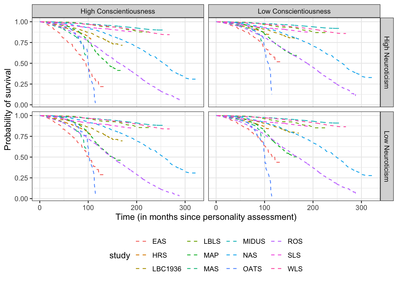
Survival plots by study (time since baseline as metric)
This document contains the survival plots of the surivival models, using time since baseline as the metric of interest and neuroticism by conscientiousness as the predictor of interest.
Code
The following packages were used to generate this table:
library(papaja)
library(tidyverse)
library(knitr)
library(kableExtra)
library(here)
The files needed for this table are available at osf.io/mzfu9 in the Individual Study Output folder.
First we load the individual study analysis objects.
study.names = c("EAS", "HRS", "LBC", "LBLS", "MAP", "MAS", "MIDUS", "NAS", "OATS", "ROS", "SLS", "WLS")
lapply(here(paste0("mortality/study output/", study.names, "_survival_output.Rdata")), load, .GlobalEnv)
Next we extract the predicted values from each object.
plottime.s = lapply(paste0(study.names, "_survival_output"),
                  FUN = function(x) get(x)$plotdata$time.s) %>%
  map2_df(., study.names, ~ mutate(.x, study = .y))

plot_n = data.frame(study = study.names,
                    n = sapply(paste0(study.names, "_survival_output"),
                  FUN = function(x) get(x)$time$model2$ntotal))

plottime.s = plottime.s %>%
  full_join(plot_n)
Finally, we plot individual values, as well as the overall weighted line.
plottime.s %>%
  mutate(study = gsub("LBC", "LBC1936", study)) %>%
  mutate(z.neur = factor(z.neur, levels = c(-1, 1), labels = c("High Neuroticism", "Low Neuroticism")),
         z.con = factor(z.con, levels = c(-1, 1), labels = c("High Conscientiousness", "Low Conscientiousness"))) %>%
  ggplot(aes(x = time, y = probability)) +
  geom_line(aes(color = study), linetype = "dashed") +
  # stat_smooth(aes(weight = n),
  #             method = "loess",
  #             formula = y ~ x,
  #             se =  TRUE,
  #             size = 1, color = "black") +
  scale_x_continuous("Time (in months since personality assessment)") +
  scale_y_continuous("Probability of survival") +
  facet_grid(z.neur~z.con) +
  theme_bw() +
  theme(legend.position = "bottom")