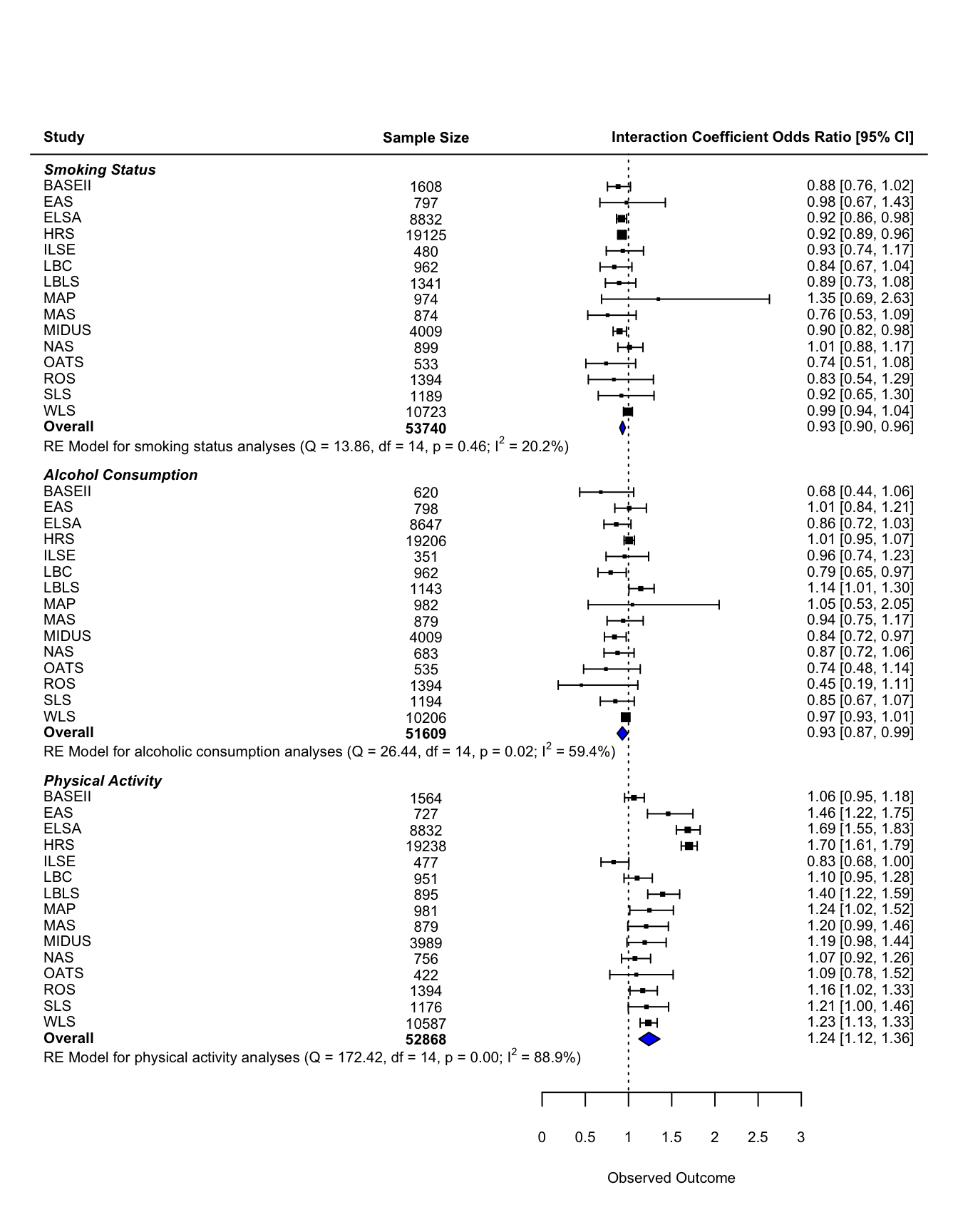
Forest Plot (main effect of conscientiousness)
This document contains the forest plot summarizing the analyses described in the manuscript.
Code
The following packages were used to generate this figure:
library(tidyverse)
library(metafor)
library(papaja)
library(here)
The files needed for this table are available at osf.io/mzfu9 in the Meta Analysis Output folder.
First we load the meta-analysis objects. As we load them in, we rename some of the objects (as they were given the same name during creation).
load(here("behavior/created data/meta_smoker_main.Rdata"))
load(here("behavior/created data/meta_drinker_main.Rdata"))
load(here("behavior/created data/meta_active_main.Rdata"))
The data frames contain the estimates and standard errors for each study, as well as confidence intervals. We bind these into a single large data frame.
smoker.main.data <- smoker.main.data %>%
  mutate(outcome = "smoker")

drinker.main.data <- drinker.main.data %>%
  mutate(outcome = "drinker")

active.main.data <- active.main.data %>%
  mutate(outcome = "active")

data_main_all <- smoker.main.data %>%
  full_join(drinker.main.data) %>%
  full_join(active.main.data) %>%
  mutate(n = printnum(n)) #format as integer with commas
Next we calculate the bounds of the figure (along the x-axis), based on the data we know will be plotted. Then we use the known bounds to point to where we want the extra information. For this figure, extra information is just the sample size.
  # find maximum upper bound of confidence intervals
max.ci.main = max(exp(data_main_all$con_estimate + 1.96*data_main_all$con_std.error))
  # find minimum lower bound of confidence intervals
min.ci.main = min(exp(data_main_all$con_estimate - 1.96*data_main_all$con_std.error))

range.main = max.ci.main-min.ci.main

#give some space on either side. These are the plot bounds
lower.main = min.ci.main-(range.main)
upper.main = max.ci.main+(range.main)

#estimate position of extra information
lower.main = min.ci.main-(range.main*2.5)
upper.main = max.ci.main+(range.main*.75)

#estimate position of extra information
  # range of space between left side of plot and lowerbound of confidence intervals
pos.main = min.ci.main-lower.main
  # break that into equal sections.
pos.main = pos.main/4
  #use the sections for figure out where you want each column to be in that space
pos.main = c(lower.main+3*pos.main)
Now we calculated the needed space along the y-axis. First we determine how many extra rows we need between each “set” of analyses (in this case, between each chronic condition). We need two extra rows for specific information: the weighted average estimates and a label. From there, I added extra rows until the figure looked appealing. I ended up with 5 extra rows.
From there, I figure out which rows will be filled with each set of analyses. It’s important to remember that rows start from the bottom and as you move up the figure, the row number increases.
extra.space = 5

# which rows are for active disease
total.active = nrow(active.main.data)
rows.active = c(1, total.active)

# which rows are for drinker
total.drinker = nrow(drinker.main.data)
# skip row for drinker summary, space, and active title
rows.drinker = c(rows.active[2] + extra.space, rows.active[2] + extra.space + total.drinker - 1)

# which rows are for highblood pressure
total.smoker = nrow(smoker.main.data)
# skip row for smoker summary, space, title
rows.smoker = c(rows.drinker[2] + extra.space, rows.drinker[2] + extra.space + total.smoker - 1)
The last step before beginning the plot is to set the font size and formatting. font = 1 is the non-bold, non-italic font.
cex.value = .65
par(font = 1)
The final chunck builds the forest plot. Comments are included throughout as a guide.
forest(data_main_all$con_estimate, #estimate
       data_main_all$con_std.error^2, #variance
       xlim = c(lower.main, upper.main), #limits of x-axis, full figure
       ylim = c(-1, nrow(data_main_all) + extra.space*2 + 2), # limits of y-axis
       cex = cex.value, #font size
       slab = data_main_all$study, #study label
       transf=exp, #transformation to estimates (takes from log odds to odds ratio)
       refline = 1, # where is the vertical line representing the null?
       # which rows do I fill in. Remember, data frame goes from top to bottom, but row numbers on
       # figure go from bottom to top
       rows = c(rows.smoker[2]:rows.smoker[1],
                rows.drinker[2]:rows.drinker[1],
                rows.active[2]:rows.active[1]),
       # what extra information is added?
       ilab = data_main_all[,c("n")],
       # where does extra information go?
       ilab.xpos = pos.main)

# add weighted average effects polygon
addpoly(smoker.main_c.rma, row=rows.smoker[1]-1, cex = cex.value, transf = exp, mlab = "", col = "blue")
addpoly(drinker.main_c.rma, row=rows.drinker[1]-1, cex = cex.value, transf = exp, mlab = "", col = "blue")
addpoly(active.main_c.rma, row=rows.active[1]-1, cex = cex.value, transf = exp, mlab = "", col = "blue")

### add text with Q-value, dfs, p-value, and I^2 statistic for subgroups
text(x = lower.main, y = rows.smoker[1]-2.25, pos=4, cex = cex.value,
     bquote(paste("RE Model for smoking status analyses (Q = ",
                  .(formatC(smoker.main_c.rma$QE, digits=2, format="f")),
                  ", df = ", .(smoker.main_c.rma$k - smoker.main_c.rma$p),
                  ", p = ", .(formatC(smoker.main_c.rma$QEp, digits=2, format="f")), "; ", I^2, " = ",
                  .(formatC(smoker.main_c.rma$I2, digits=1, format="f")), "%)")))
text(x = lower.main, y = rows.drinker[1]-2.25, pos=4, cex = cex.value,
     bquote(paste("RE Model for alcoholic consumption analyses (Q = ",
                  .(formatC(drinker.main_c.rma$QE, digits=2, format="f")),
                  ", df = ", .(drinker.main_c.rma$k - drinker.main_c.rma$p),
                  ", p = ", .(formatC(drinker.main_c.rma$QEp, digits=2, format="f")), "; ", I^2, " = ",
                  .(formatC(drinker.main_c.rma$I2, digits=1, format="f")), "%)")))
text(x = lower.main, y = rows.active[1]-2.25, pos=4, cex = cex.value,
     bquote(paste("RE Model for physical activity analyses (Q = ",
                  .(formatC(active.main_c.rma$QE, digits=2, format="f")),
                  ", df = ", .(active.main_c.rma$k - active.main_c.rma$p),
                  ", p = ", .(formatC(active.main_c.rma$QEp, digits=2, format="f")), "; ", I^2, " = ",
                  .(formatC(active.main_c.rma$I2, digits=1, format="f")), "%)")))

#bold font
par(font = 2)

# add "overall"" label to each set of analyses
text(lower.main, y = c(rows.smoker[1]-1, rows.drinker[1]-1, rows.active[1]-1), pos = 4, cex = cex.value, "Overall")

# add overall sample sizes for each set of analyses
text(x = pos.main[1], y = rows.smoker[1]-1, cex = cex.value, printnum(sum(smoker.main.data$n)))
text(x = pos.main[1], y = rows.drinker[1]-1, cex = cex.value, printnum(sum(drinker.main.data$n)))
text(x = pos.main[1], y = rows.active[1]-1, cex = cex.value, printnum(sum(active.main.data$n)))


# column labels
text(lower.main, nrow(data_main_all) + extra.space*2 + 1,
     "Study", cex = cex.value, pos = 4)
text(upper.main, nrow(data_main_all) + extra.space*2 + 1,
     "Interaction Coefficient Odds Ratio [95% CI]", cex = cex.value, pos=2)
text(pos.main[1], nrow(data_main_all) + extra.space*2 + 1,
     "Sample Size", cex = cex.value)
text((pos.main[2]+pos.main[3])/2, nrow(data_main_all) + extra.space*2 + 2,
     "conscientiousness Coefficient", cex = cex.value)

#bold and italic font, plus bigger text
par(font = 4)

# outcome labels
text(lower.main, rows.smoker[2] + 1,
     "Smoking Status", cex = cex.value, pos = 4)
text(lower.main, rows.drinker[2] + 1,
     "Alcohol Consumption", cex = cex.value, pos = 4)
text(lower.main, rows.active[2] + 1,
     "Physical Activity", cex = cex.value, pos = 4)