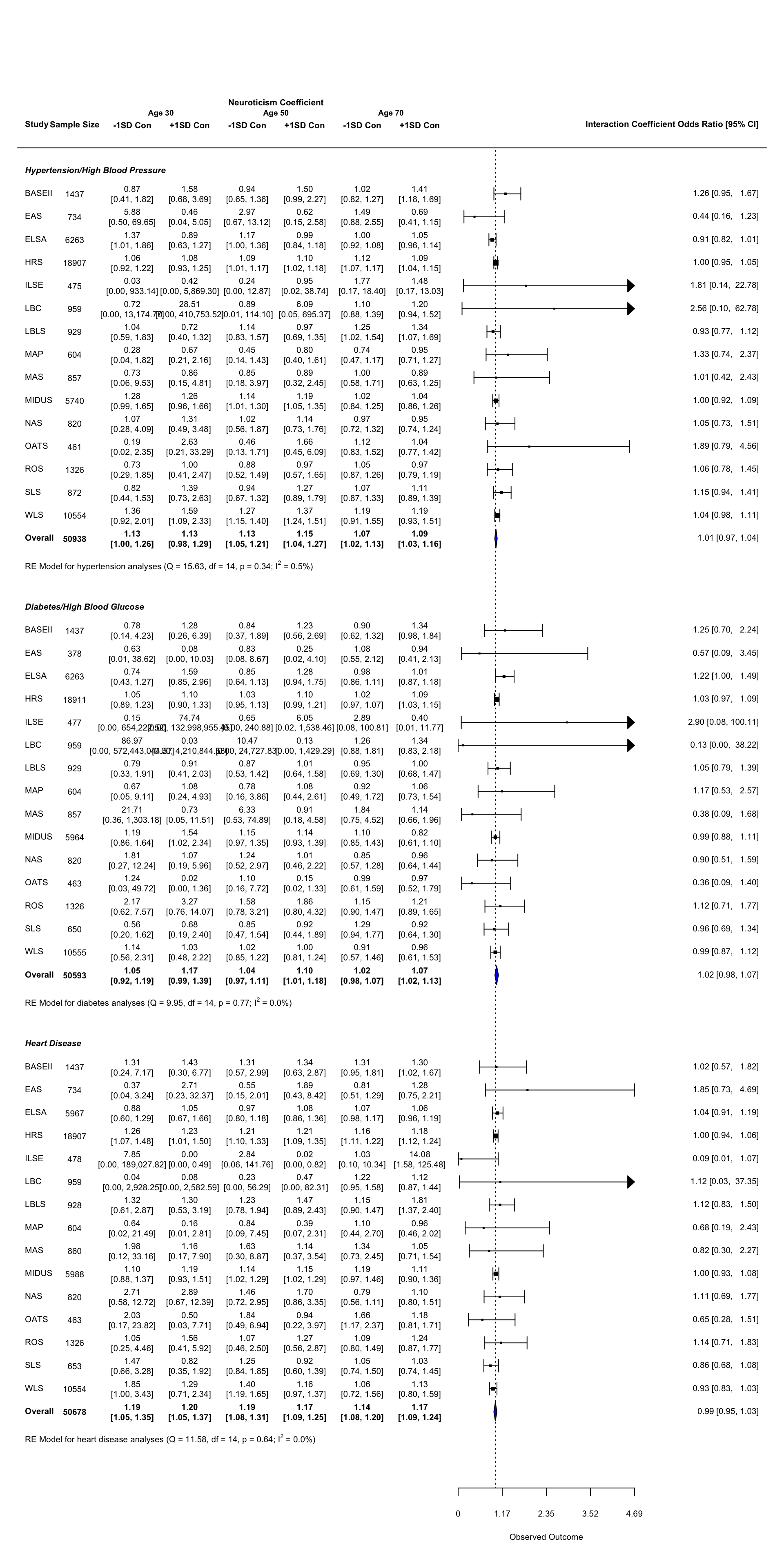
Forest Plot: Age by Neuroticism by Conscientiousness (Cross Sectional Analyses)
This document contains the forest plot summarizing the relationship between the 3-way interaction of age, neuroticism and conscientiousness and concurrent health condition status. These analyses were not preregistered and are exploratory.
Code
The following packages were used to generate this figure:
library(tidyverse)
library(metafor)
library(papaja)
library(here)
The files needed for this table are available at osf.io/mzfu9 in the Meta Analysis Output folder.
First we load the meta-analysis objects. As we load them in, we rename some of the objects (as they were given the same name during creation).
load(here("chronic/meta output/hbp_cross_age.Rdata"))
meta.cross.hbp = meta.int.mod3
lowc_30_ci.hbp = meta_lowc_30_ci_mod3
hghc_30_ci.hbp = meta_hghc_30_ci_mod3
lowc_50_ci.hbp = meta_lowc_50_ci_mod3
hghc_50_ci.hbp = meta_hghc_50_ci_mod3
lowc_70_ci.hbp = meta_lowc_70_ci_mod3
hghc_70_ci.hbp = meta_hghc_70_ci_mod3

load(here("chronic/meta output/diabetes_cross_age.Rdata"))
meta.cross.diabetes = meta.int.mod3
lowc_30_ci.diab = meta_lowc_30_ci_mod3
hghc_30_ci.diab = meta_hghc_30_ci_mod3
lowc_50_ci.diab = meta_lowc_50_ci_mod3
hghc_50_ci.diab = meta_hghc_50_ci_mod3
lowc_70_ci.diab = meta_lowc_70_ci_mod3
hghc_70_ci.diab = meta_hghc_70_ci_mod3

load(here("chronic/meta output/heart_cross_age.Rdata"))
meta.cross.heart = meta.int.mod3
lowc_30_ci.heart = meta_lowc_30_ci_mod3
hghc_30_ci.heart = meta_hghc_30_ci_mod3
lowc_50_ci.heart = meta_lowc_50_ci_mod3
hghc_50_ci.heart = meta_hghc_50_ci_mod3
lowc_70_ci.heart = meta_lowc_70_ci_mod3
hghc_70_ci.heart = meta_hghc_70_ci_mod3

rm(meta.int.mod3)
rm(meta_lowc_30_ci_mod3)
rm(meta_hghc_30_ci_mod3)
rm(meta_lowc_50_ci_mod3)
rm(meta_hghc_50_ci_mod3)
rm(meta_lowc_70_ci_mod3)
rm(meta_hghc_70_ci_mod3)
The data frames contain the estimates and standard errors for each study, as well as confidence intervals. We bind these into a single large data frame.
data_cross_hbp <- data_cross_hbp %>%
  # select relevant variables
  dplyr::select(contains("name"), contains("mod3")) %>%
  # add column to indicate outcome
  mutate(outcome = "hbp")

data_cross_diab <- data_cross_diab %>%
  # select relevant variables
  dplyr::select(contains("name"), contains("mod3")) %>%
  # add column to indicate outcome
  mutate(outcome = "diabetes")

data_cross_heart <- data_cross_heart %>%
  # select relevant variables
  dplyr::select(contains("name"), contains("mod3")) %>%
  # add column to indicate outcome
  mutate(outcome = "heart")

data_cross_all <- data_cross_hbp %>%
  full_join(data_cross_diab) %>%
  full_join(data_cross_heart) %>%
  mutate(n_mod3 = printnum(n_mod3, int=T)) #format as integer with commas
Next we calculate the bounds of the figure (along the x-axis), based on the data we know will be plotted. Then we use the known bounds to point to where we want the extra information. For this figure, extra information is the sample size, the estimate and confidence interval of the simple slopes of neuroticism at ±1SD conscientiousness.
  # find maximum upper bound of confidence intervals
max.ci.cross = exp(data_cross_all$int_est_mod3 + 1.96*data_cross_all$int_se_mod3)
max.ci.cross = max.ci.cross[order(max.ci.cross, decreasing = T)][6]
  # find minimum lower bound of confidence intervals
min.ci.cross = min(exp(data_cross_all$int_est_mod3 - 1.96*data_cross_all$int_se_mod3))

range.cross = max.ci.cross-min.ci.cross

#estimate position of extra information
lower.cross = min.ci.cross-(range.cross*2.5)
upper.cross = max.ci.cross+(range.cross*.75)

#estimate position of extra information
  # range of space between left side of plot and lowerbound of confidence intervals
pos.cross = min.ci.cross-lower.cross
  # break that into equal sections. I find that 11 works for one column of sample
  # sizes and two columns of estimates and confidence intervals
pos.cross = pos.cross/23
  #use the sections for figure out where you want each column to be in that space
pos.cross = c(lower.cross+3*pos.cross,
             lower.cross+6*pos.cross,
             lower.cross+9*pos.cross,
             lower.cross+12*pos.cross,
             lower.cross+15*pos.cross,
             lower.cross+18*pos.cross,
             lower.cross+21*pos.cross)
Now we calculated the needed space along the y-axis. First we determine how many extra rows we need between each “set” of analyses (in this case, between each chronic condition). We need two extra rows for specific information: the weighted average estimates and a label. From there, I added extra rows until the figure looked appealing. I ended up with 5 extra rows.
From there, I figure out which rows will be filled with each set of analyses. It’s important to remember that rows start from the bottom and as you move up the figure, the row number increases.
extra.space = 5

# which rows are for heart disease
total.heart = nrow(data_cross_heart)
rows.heart = c(1, total.heart)

# which rows are for diabetes
total.diabetes = nrow(data_cross_diab)
# skip row for diabetes summary, space, and heart title
rows.diabetes = c(rows.heart[2] + extra.space, rows.heart[2] + extra.space + total.diabetes - 1)

# which rows are for highblood pressure
total.hbp = nrow(data_cross_hbp)
# skip row for hbp summary, space, title
rows.hbp = c(rows.diabetes[2] + extra.space, rows.diabetes[2] + extra.space + total.hbp - 1)
The last step before beginning the plot is to set the font size and formatting. font = 1 is the non-bold, non-italic font.
cex.value = .65
par(font = 1)
The final chunck builds the forest plot. Comments are included throughout as a guide.
forest(data_cross_all$int_est_mod3, #estimate
       data_cross_all$int_se_mod3^2, #variance
       xlim = c(lower.cross, upper.cross), #limits of x-axis, full figure
       alim = c(min.ci.cross, max.ci.cross),
       ylim = c(-1, nrow(data_cross_all) + extra.space*2 + 2), # limits of y-axis
       cex = cex.value, #font size
       slab = data_cross_all$name, #study label
       transf=exp, #transformation to estimates (takes from log odds to odds ratio)
       refline = 1, # where is the vertical line representing the null?
       # which rows do I fill in. Remember, data frame goes from top to bottom, but row numbers on
       # figure go from bottom to top
       rows = c(rows.hbp[2]:rows.hbp[1],
                rows.diabetes[2]:rows.diabetes[1],
                rows.heart[2]:rows.heart[1]),
       # what extra information is added?
       ilab = data_cross_all[,c("n_mod3",
                                 "neur_lowc_30_ci_mod3",
                                 "neur_hghc_30_ci_mod3",
                                 "neur_lowc_50_ci_mod3",
                                 "neur_hghc_50_ci_mod3",
                                 "neur_lowc_70_ci_mod3",
                                 "neur_hghc_70_ci_mod3")],
       # where does extra information go?
       ilab.xpos = pos.cross)

# add weighted average effects polygon
addpoly(meta.cross.hbp, row=rows.hbp[1]-1, cex = cex.value, transf = exp, mlab = "", col = "blue")
addpoly(meta.cross.diabetes, row=rows.diabetes[1]-1, cex = cex.value, transf = exp, mlab = "", col = "blue")
addpoly(meta.cross.heart, row=rows.heart[1]-1, cex = cex.value, transf = exp, mlab = "", col = "blue")

### add text with Q-value, dfs, p-value, and I^2 statistic for subgroups
text(x = lower.cross, y = rows.hbp[1]-2.25, pos=4, cex = cex.value,
     bquote(paste("RE Model for hypertension analyses (Q = ",
                  .(formatC(meta.cross.hbp$QE, digits=2, format="f")),
                  ", df = ", .(meta.cross.hbp$k - meta.cross.hbp$p),
                  ", p = ", .(formatC(meta.cross.hbp$QEp, digits=2, format="f")), "; ", I^2, " = ",
                  .(formatC(meta.cross.hbp$I2, digits=1, format="f")), "%)")))
text(x = lower.cross, y = rows.diabetes[1]-2.25, pos=4, cex = cex.value,
     bquote(paste("RE Model for diabetes analyses (Q = ",
                  .(formatC(meta.cross.diabetes$QE, digits=2, format="f")),
                  ", df = ", .(meta.cross.diabetes$k - meta.cross.diabetes$p),
                  ", p = ", .(formatC(meta.cross.diabetes$QEp, digits=2, format="f")), "; ", I^2, " = ",
                  .(formatC(meta.cross.diabetes$I2, digits=1, format="f")), "%)")))
text(x = lower.cross, y = rows.heart[1]-2.25, pos=4, cex = cex.value,
     bquote(paste("RE Model for heart disease analyses (Q = ",
                  .(formatC(meta.cross.heart$QE, digits=2, format="f")),
                  ", df = ", .(meta.cross.heart$k - meta.cross.heart$p),
                  ", p = ", .(formatC(meta.cross.heart$QEp, digits=2, format="f")), "; ", I^2, " = ",
                  .(formatC(meta.cross.heart$I2, digits=1, format="f")), "%)")))

#bold font
par(font = 2)

# add "overall"" label to each set of analyses
text(lower.cross, y = c(rows.hbp[1]-1, rows.diabetes[1]-1, rows.heart[1]-1), pos = 4, cex = cex.value, "Overall")

# add overall sample sizes for each set of analyses
text(x = pos.cross[1], y = rows.hbp[1]-1, cex = cex.value, printnum(sum(data_cross_hbp$n_mod3), int=T))
text(x = pos.cross[1], y = rows.diabetes[1]-1, cex = cex.value, printnum(sum(data_cross_diab$n_mod3), int = T))
text(x = pos.cross[1], y = rows.heart[1]-1, cex = cex.value, printnum(sum(data_cross_heart$n_mod3), int =T))
#
# add weighted average simple slopes for each set of analyses
text(x = pos.cross[2:7], y = rows.hbp[1]-1, cex = cex.value, c(lowc_30_ci.hbp, hghc_30_ci.hbp,
                                                               lowc_50_ci.hbp, hghc_50_ci.hbp,
                                                               lowc_70_ci.hbp, hghc_70_ci.hbp))

text(x = pos.cross[2:7], y = rows.diabetes[1]-1, cex = cex.value, c(lowc_30_ci.diab, hghc_30_ci.diab,
                                                                    lowc_50_ci.diab, hghc_50_ci.diab,
                                                                    lowc_70_ci.diab, hghc_70_ci.diab))

text(x = pos.cross[2:7], y = rows.heart[1]-1, cex = cex.value, c(lowc_30_ci.heart, hghc_30_ci.heart,
                                                               lowc_50_ci.heart, hghc_50_ci.heart,
                                                               lowc_70_ci.heart, hghc_70_ci.heart))


# column labels
text(lower.cross, nrow(data_cross_all) + extra.space*2 + 1,
     "Study", cex = cex.value, pos = 4)
text(upper.cross, nrow(data_cross_all) + extra.space*2 + 1,
     "Interaction Coefficient Odds Ratio [95% CI]", cex = cex.value, pos=2)
text(pos.cross[1], nrow(data_cross_all) + extra.space*2 + 1,
     "Sample Size", cex = cex.value)
text(c((pos.cross[2]+pos.cross[3])/2, (pos.cross[4]+pos.cross[5])/2, (pos.cross[6]+pos.cross[7])/2),
     nrow(data_cross_all) + extra.space*2 + 1.5,
     c("Age 30", "Age 50", "Age 70"), cex = .6)

text(pos.cross[c(2,4,6)], nrow(data_cross_all) + extra.space*2 + 1,
     "-1SD Con", cex = cex.value)
text(pos.cross[c(3,5,7)], nrow(data_cross_all) + extra.space*2 + 1,
     "+1SD Con", cex = cex.value)
text((pos.cross[2]+pos.cross[7])/2, nrow(data_cross_all) + extra.space*2 + 2,
     "Neuroticism Coefficient", cex = cex.value)

#bold and italic font, plus bigger text
par(font = 4)

# outcome labels
text(lower.cross, rows.hbp[2] + 1,
     "Hypertension/High Blood Pressure", cex = cex.value, pos = 4)
text(lower.cross, rows.diabetes[2] + 1,
     "Diabetes/High Blood Glucose", cex = cex.value, pos = 4)
text(lower.cross, rows.heart[2] + 1,
     "Heart Disease", cex = cex.value, pos = 4)