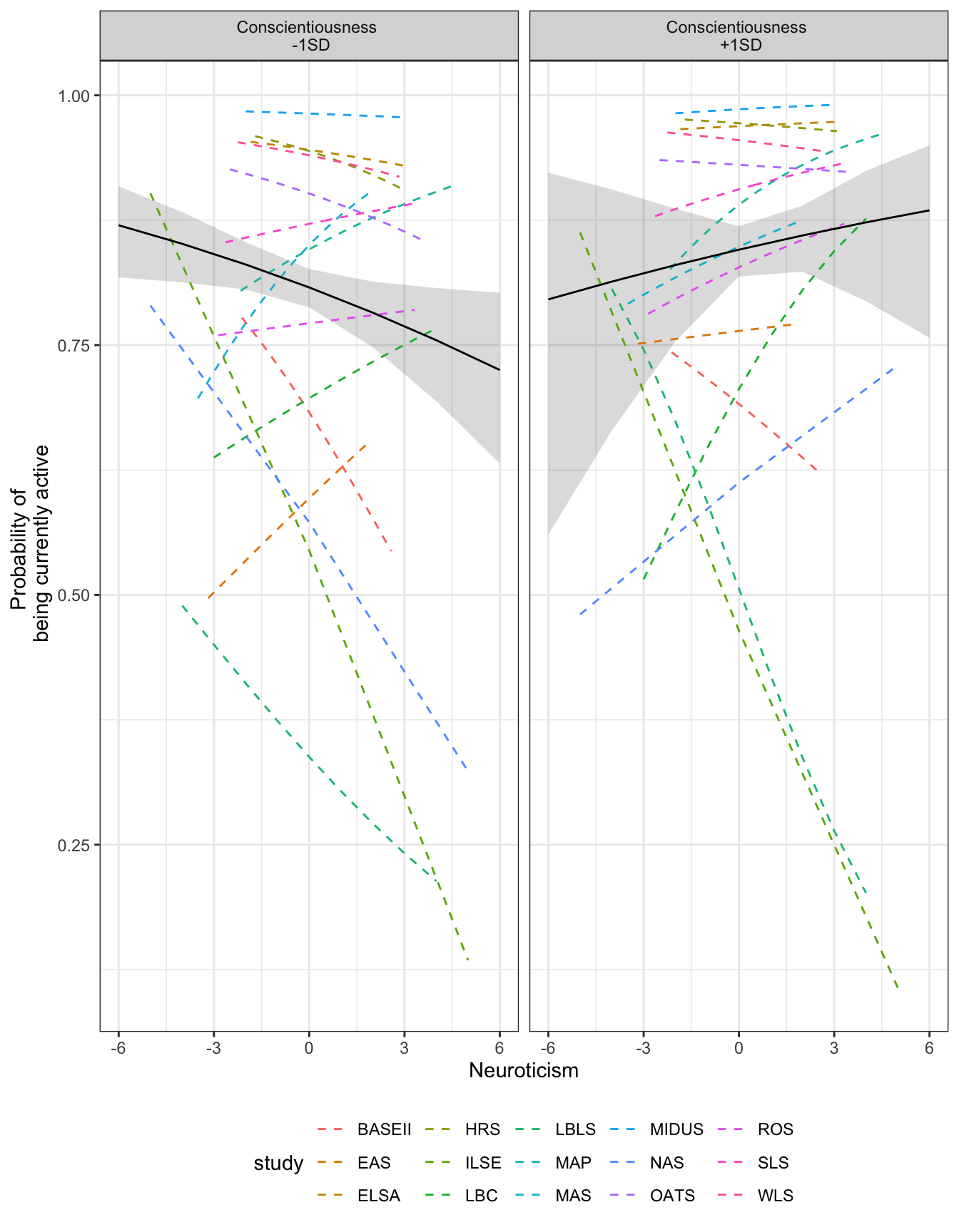
Predicted Values: Physical activity status
This document contains the plot of predicted probabilities from each individual study, as well as the weighted average effect, from the cross-sectional analyses.
Code
The following packages were used to generate this figure:
library(tidyverse)
library(metafor)
library(here)
The files needed for this table are available at osf.io/mzfu9 in the Meta Analysis Output folder.
First we load the meta-analysis objects. To see how these objects were created, see the meta-analysis script titled active_meta-analysis.R that are available at osf.io/zvsfb.
load(here("behavior/created data/plot_active.Rdata"))We plot the values.
active.plot %>%
  ggplot(., aes(x = x, y = predicted)) +
  geom_ribbon(aes(ymin=lower, ymax=upper), fill="black", alpha=.15,
              data = weighted.vals)+
  geom_line(aes(color = study), lty="dashed") +
  geom_line(data = weighted.vals, color="black") +
  scale_x_continuous("Neuroticism")+
  scale_y_continuous("Probability of \n being currently active") +
  facet_wrap(~group) +
  theme_bw() +
  theme(legend.position = "bottom")