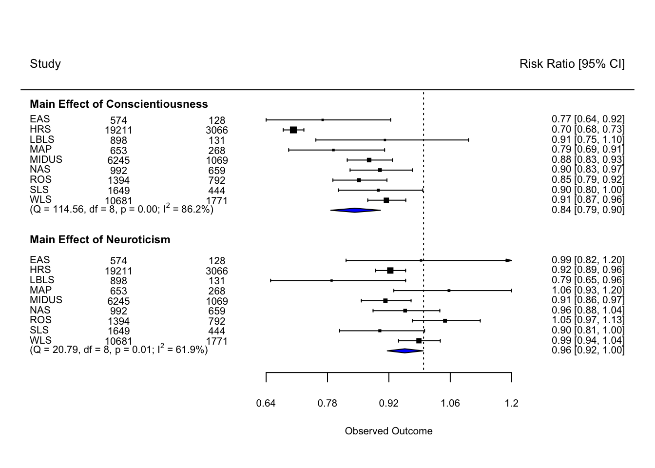
Meta analysis of main effects of neuroticism and conscientiousness (time since baseline as metric)
This document contains the meta-analysis of the surivival models, using time since baseline as the metric of interest and neuroticism by conscientiousness as the predictor of interest.
Please note these models were developed after peer review – they do not appear in our preregistration. In addition, there have been some difficulties in estimating the models in all datasets. The information provided here is our most up-to-date version; these analyses were performed on 2020-02-13
save(meta.results.time.neur, file = here("morality/created data/main_effects_neur.Rdata"))
save(meta.results.time.con,  file = here("morality/created data/main_effects_con.Rdata"))
Code
The following packages were used to generate this table:
library(papaja)
library(tidyverse)
library(metafor)
library(knitr)
library(kableExtra)
library(here)
Specify the location of the study analysis objects. The first author stored these in a Box Sync folder, but you may have downloaded these to a different location. The files needed for this table are available at osf.io/mzfu9 in the Individual Study Output folder.
data.path = here("mortality/study output/")First we load the individual study analysis objects.
study.names = c("EAS", "HRS","LBLS", "MAP", "MIDUS", "NAS", "ROS", "SLS", "WLS")

lapply(paste0(data.path, study.names, "_survival_output.Rdata"), load, .GlobalEnv)
meta.data.time <- data.frame()
n <- 0
for(i in study.names){
n <- n+1
x <- get(paste0(i, "_survival_output"))
meta.data.time[n, "study"] <- i
meta.data.time[n, "n_coef"] <- x$time$model0a$coef["z.neur", "coef"]
meta.data.time[n, "n_se"] <- x$time$model0a$coef["z.neur", "se(coef)"]
meta.data.time[n, "c_coef"] <- x$time$model0a$coef["z.con", "coef"]
meta.data.time[n, "c_se"] <- x$time$model0a$coef["z.con", "se(coef)"]
meta.data.time[n, "n"] <- x$time$model0a$ntotal
meta.data.time[n, "n_died"] <- x$descriptives$died.tab["1"]
}
meta.results.time.neur <- rma(yi = n_coef,
sei = n_se,
ni = n,
measure = "RR",
slab = study,
data = meta.data.time)
meta.results.time.con <- rma(yi = c_coef,
sei = c_se,
ni = n,
measure = "RR",
slab = study,
data = meta.data.time)
meta.data.time = meta.data.time %>%
gather("key", "value", n_coef, n_se, c_coef, c_se) %>%
separate("key", into = c("trait", "key")) %>%
spread("key", "value")
meta.results.time = rma(yi = coef,
sei = se,
ni = n,
measure = "RR",
slab = study,
data = meta.data.time)meta.data.time = meta.data.time %>%
#mutate(study = gsub("LBC", "LBC1936", study)) %>%
arrange(trait, study)
#find plot limits
max.ci = meta.data.time %>%
mutate(ci = exp(coef+1.96*se)) %>%
arrange(desc(ci))
max.ci = max.ci[2, "ci"]
#max.ci = max(exp(neur.data$estimate+1.96*neur.data$se))
min.ci = min(exp(meta.data.time$coef-1.96*meta.data.time$se))
range = max.ci-min.ci
lower = min.ci-(range)
upper = max.ci+(range)*.5
#estimate position of extra information
pos = min.ci-lower
pos = pos/2
pos = c(lower+.8*pos, lower+1.6*pos)
unique = nrow(meta.data.time)/2
rows = c(1:unique, (unique+6):((2*unique)+5))
cex.set = .65
forest(meta.data.time$coef, meta.data.time$se^2,
cex = cex.set,
slab = meta.data.time$study,
xlim = c(lower, upper),
alim = c(min.ci, max.ci),
transf=exp,
rows = rows[order(rows,decreasing = T)],
ylim = c(-1, 5+max(rows)),
refline = 1,
ilab = meta.data.time[,c("n", "n_died")],
ilab.xpos = pos)
addpoly(meta.results.time.con, row = unique+5,
cex = cex.set,transf =exp, mlab="", col = "blue")
addpoly(meta.results.time.neur, row = min(rows)-1,
cex = cex.set,transf =exp, mlab="", col = "blue")
text(lower, unique+5, pos=4, cex = cex.set,
bquote(paste("(Q = ",
.(formatC(meta.results.time.con$QE, digits=2, format="f")),
", df = ", .(meta.results.time.con$k - meta.results.time.con$p),
", p = ", .(formatC(meta.results.time.con$QEp, digits=2, format="f")),
"; ", I^2, " = ",
.(formatC(meta.results.time.con$I2, digits=1, format="f")), "%)")))
text(lower, min(rows)-1, pos=4, cex = cex.set,
bquote(paste("(Q = ",
.(formatC(meta.results.time.neur$QE, digits=2, format="f")),
", df = ", .(meta.results.time.neur$k - meta.results.time.neur$p),
", p = ", .(formatC(meta.results.time.neur$QEp, digits=2, format="f")),
"; ", I^2, " = ",
.(formatC(meta.results.time.neur$I2, digits=1, format="f")), "%)")))
text(lower, 5.5+max(rows),
"Study", cex = cex.set*1.2, pos = 4)
text(upper, 5.5+max(rows),
"Risk Ratio [95% CI]", cex = cex.set*1.2, pos=2)
text(lower, max(rows)+1.5,
"Main Effect of Conscientiousness", cex = cex.set*1.1, pos = 4, font = 2)
text(lower, unique+2,
"Main Effect of Neuroticism", cex = cex.set*1.1, pos = 4, font = 2)